Computer simulations of the climate system, built from physical laws and used to understand past climate and project future change. They are the principal tool of the field and their limitations are specific and well characterised.
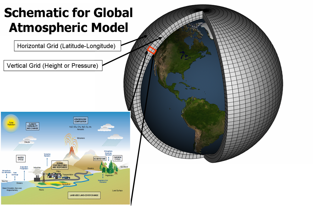
A climate model divides the atmosphere and ocean into a three-dimensional grid of cells and solves equations for each: conservation of mass, momentum and energy, together with the behaviour of water in its three phases.
The calculation proceeds in time steps, with the state of each cell at one step determining the next.
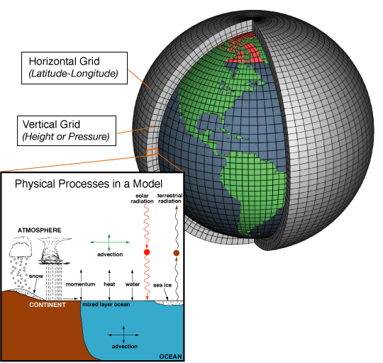
Modern models are coupled, meaning separate components for atmosphere, ocean, land surface and sea ice run together and exchange energy, water and momentum at their interfaces. Earth system models add carbon cycle, vegetation and atmospheric chemistry.
The physics is not adjusted to produce a desired answer. Most of what a model contains is the same fluid dynamics and radiative transfer used in weather forecasting, and much of the code is shared.
Grid cells are large, typically tens to a hundred kilometres across in global models. Many important processes occur at much smaller scales.
Cloud formation, convection, turbulence and precipitation all happen well below grid resolution. They cannot be resolved, so they are parameterised: represented by relationships that express their aggregate effect in terms of the resolved variables.
Parameterisation is where models differ most and where most of their uncertainty originates. Clouds are the principal case, since they both reflect sunlight and trap outgoing radiation, and their net effect depends on type, altitude and extent.
This is the honest statement of the field's central uncertainty. Climate sensitivity, the warming resulting from a doubling of carbon dioxide, has a range that is driven substantially by how clouds respond, and the climate sensitivity capsule treats it.
Models are evaluated against observations they were not built to reproduce, which is the relevant test.
Historical simulation runs a model over the instrumental period using known changes in greenhouse gases, aerosols, solar output and volcanic eruptions, and compares the result with the observed record.
Volcanic eruptions provide sharp tests. The eruption of Pinatubo in 1991 injected sulphate aerosols into the stratosphere, and models predicted the magnitude and duration of the resulting cooling before the observations were in.
Palaeoclimate simulation tests models against conditions very different from the present, including the last glacial maximum and warm periods millions of years ago.
Emergent properties are a further test. Models are not tuned to produce El Nino, monsoons, storm tracks or the seasonal cycle, and they generate them, which indicates the underlying physics is behaving correctly.
Retrospective assessment of published projections has found that models from the 1970s onward projected subsequent warming with reasonable accuracy once actual rather than assumed emissions are used, which is the appropriate comparison.
Global mean temperature response to a given emissions path is the quantity models handle best, and agreement between independent models is close.
Large-scale patterns, including greater warming over land than ocean, amplified warming in the Arctic, and intensification of the water cycle, are robust across models and are observed.
Regional detail is much weaker. Projections of precipitation change at the scale of a country or a river basin differ substantially between models, and this is the honest limitation for anyone seeking local guidance.
Abrupt changes and tipping elements are represented poorly, since the processes involved often operate below grid scale or are not included at all.
Models do not predict the future in the sense of forecasting. They project what follows from specified assumptions about emissions, and the emissions themselves are a social and political variable that no physical model can supply.
Ensembles are the standard approach. Running many models, or one model many times with slightly different initial conditions, produces a spread that indicates how much of a result is robust and how much depends on modelling choices.
The Coupled Model Intercomparison Project coordinates this internationally, running standardised experiments across dozens of models from many institutions, and its output underpins the assessment reports.
Model spread is reported rather than hidden, and a projection stated as a range with a most likely value is the normal output format.
Climate models are the only means of answering what follows from a given emissions path, since the experiment cannot be run on the actual planet and the relevant timescales exceed any observational record.
They also demonstrate a general property of complex simulation: a model built from established physics can be genuinely predictive at some scales and unreliable at others, and knowing which is which is what distinguishes informed use from either dismissal or overconfidence.