The symmetric bell-shaped probability distribution that arises whenever many small independent influences add together. It is the most important distribution in statistics, and it is also the most frequently misapplied.
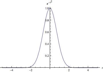
The distribution is defined by two parameters: the mean, which locates its centre, and the standard deviation, which sets its width. Every normal distribution has the same shape, differing only in position and scale.
Its most used property is how probability is distributed by distance from the centre. About sixty eight per cent of values fall within one standard deviation of the mean, about ninety five per cent within two, and about ninety nine point seven per cent within three. This is the origin of the two standard deviation convention that underlies much of applied statistics.
The tails fall away extremely rapidly. A value five standard deviations from the mean has a probability of roughly one in three and a half million, which is why events described as many standard deviations out are essentially impossible if the distribution really is normal, and why their occurrence is usually evidence that it is not.

The reason is the central limit theorem, which is treated in its own capsule. Informally, it states that the sum of many independent random influences tends toward a normal distribution regardless of how each individual influence is distributed.
This is why the distribution appears in measurement error, where many small independent errors add; in biological quantities such as height, influenced by many genetic and environmental factors; and in the average of any sample, which is why it underlies most statistical inference even when the underlying data are not normal.
The Galton board demonstrates it physically. Balls dropped through a grid of pins are deflected left or right at each level, and their accumulated positions approximate the distribution.
The theorem also explains where the distribution does not apply. If influences are not independent, or if one dominates, or if they multiply rather than add, the result is not normal. Quantities produced by multiplicative processes, including income and many biological growth measures, tend to be lognormal, meaning normal after taking logarithms, which is why income distributions are strongly skewed.
Abraham de Moivre derived the curve around 1733 as an approximation to the binomial distribution, in the context of games of chance.
Pierre-Simon Laplace developed the central limit theorem and applied the distribution broadly.
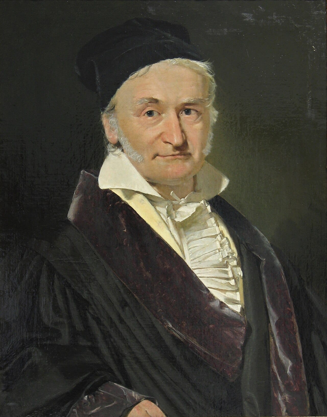
Carl Friedrich Gauss used it in 1809 in analysing errors in astronomical observation, and the association with his name has stuck, so it is often called the Gaussian distribution. This is a standard case of a result named after neither its first discoverer nor its most complete developer.
Adolphe Quetelet applied it to human characteristics in the 1830s, introducing the idea of the average man. Francis Galton developed it further and coined the term regression, and both extended the distribution into arguments about human variation and heredity that were used to support eugenics, which is part of the history of the concept and is treated in its own capsules.
The name normal is unhelpful and has consequences. It carries a suggestion that this distribution is the usual or correct one for data to follow, and the widespread assumption that data are normal unless shown otherwise is exactly the error the name invites.
The most consequential misuse is in finance. Asset returns have far fatter tails than the normal distribution allows, meaning extreme moves occur far more often than the model predicts. Risk models built on normality therefore understate the probability of large losses, and this has contributed to several financial crises, since events the models classed as near-impossible occurred repeatedly.
Benoit Mandelbrot argued from the 1960s that financial data follow heavy-tailed distributions, and the point was substantially ignored in practice for decades.
The general failure mode is assuming normality without checking. Many quantities are skewed, bounded, multimodal or heavy-tailed, and applying methods that assume normality to them produces confident and wrong answers.
Human variation is a second area of misuse. That a trait is normally distributed says nothing about the causes of that variation, and treating a bell curve as evidence about heredity or about group differences is an inference the distribution does not support.
The normal distribution is the foundation of statistical practice: significance tests, confidence intervals, regression and quality control all rest on it directly or through the central limit theorem.
Its importance is also the reason its misapplication is costly. A method that works extremely well when its assumption holds, and fails in a specific and predictable direction when it does not, is more dangerous than one that is obviously unreliable, because the failure appears only in the cases that matter most.